[예측 모델링] tensorflow 코딩 (linear함수, MSE 평가) / Dummy variable trap

1. 비어있는 데이터 확인

 

2. X 와 y 설정

 

3. 문자열 데이터를 숫자로 변경한다. (인코딩 2가지 중 택1)

 

X의 Geography는 3개로 되어있으므로 원핫인코딩 / X의 gender는 2개로 되어있으르모 레이블 인코딩

Female, Male 정렬하면 Female이 0, Male이 1이 된다. 

(원핫인코딩)

pd.get_dummies(X, columns=['Geography'])

# 원핫 인코딩한 결과의 맨 왼쪽 컬럼은 삭제를 해도 0과 1로 모두 3개 데이터표현가능.

 Dummy variable trap : 즉 맨 앞쪽 하나의 컬럼은 지워도 된다.

 0 0 1 => 0 1

 0 1 0 => 1 0

 1 0 0 => 0 0

 

X.drop('Geography_France', axis=1, inplace=True) <= 컬럼하나 삭제해도 무방

 

4. 각 데이터의 범위를 일정하게 맞춰주는 피쳐 스케일링 한다. (classicfication 2가지 중 택1) 

  # 딥러닝은 무조건 피쳐스케일링 한다.

from sklearn.preprocessing import MinMaxScaler

scaler_X = MinMaxScaler()

X = scaler_X.fit_transform(X)

 

y.values.reshape(500, 1)

 

scaler_y = MinMaxScaler()

y = scaler_y.fit_transform(y)

 

5. 학습용과 테스트용으로 나눈다. 

 

from sklearn.model_selection import train_test_split

X_train, X_test, y_train, y_test = train_test_split(X, y, test_size=0.25, random_state=50)

 

6. 딥러닝으로 모델링

import tensorflow as tf

from tensorflow.keras.models import Sequential  # Sequential: 딥러닝 그물망 구조

from tensorflow.keras.layers import Dense  # Dense: 레이어 한 열을 말한다. 

 

model = Sequential()

 

# 첫번째 히든레이어 생성 : 이때는 인풋 레이어의 숫자도 세팅해준다. (X_train의 컬럼수)

model.add(Dense(units=6, activation='relu', input_dim= 11 ))

 

# 두번째 히든레이어 생성

model.add(Dense(units=8, activation='relu'))

 

# 아웃풋 레이어 생성

# 리그레션 문제의 액티베이션 펑션은 linear사용

model.add(Dense(units=1, activation='linear'))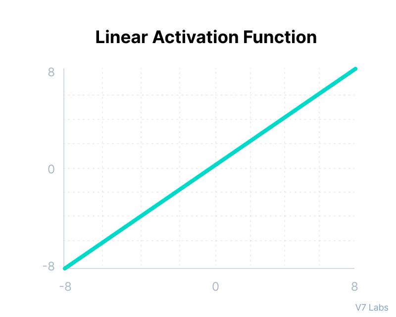

model.summary()

 

 

# 컴파일 한다! Compile한다. 오차함수를 설정하고, 옵티마이저(그레이언트 디센트 알고리즘)를 설정한다. 

model.compile(optimizer='adam', loss='mean_squared_error')

(응용)

model.compile(optimizer='adam', loss='mse', metrics=['mse','mae'])

 

# 학습

model.fit(X_train, y_train, batch_size=20, epochs=20)

 

7. 평가

y_pred = model.predict(X_test)

 

# MSE : 오차를 구하고, 제곱한 후 평균을 구한다. 

# Mean Squared Error

((y_test - y_pred)**2).mean()

 

 

plt.plot(y_test)

plt.plot(y_pred)

plt.legend(['Real', 'Pred'])

plt.show()

# 적용

new_data = np.array([0, 38, 90000, 2000, 500000])

new_data = new_data.reshape(1,5)

new_data = scaler_X.transform(new_data)

y_pred = model.predict(new_data)

scaler_y.inverse_transform(y_pred)

 

 

# 모델링을 해주는 함수를 만든다.

# 순서만 맞으면 activation을 빼줘도 된다. 

 

def build_model() : 

  model = Sequential()

  model.add(Dense(units=64, activation='relu', input_dim= X_train.shape[1] ))

  model.add(Dense(units=64, activation='relu'))

  model.add(Dense(units=1, activation='linear'))

  model.compile(optimizer='adam', loss='mean_squared_error', metrics=['mse','mae']) # loss= 'mse'로 써도 된다.

  return model

 

model= build_model()

 

epoch_history = model.fit(X_train, y_train, epochs=1000, validation_split= 0.2)

val_loss (validation)

학습중에 epochs 한번 끝날때 마다 인공지능에게 랜덤의 데이터를 시험시켜서 확인시킴